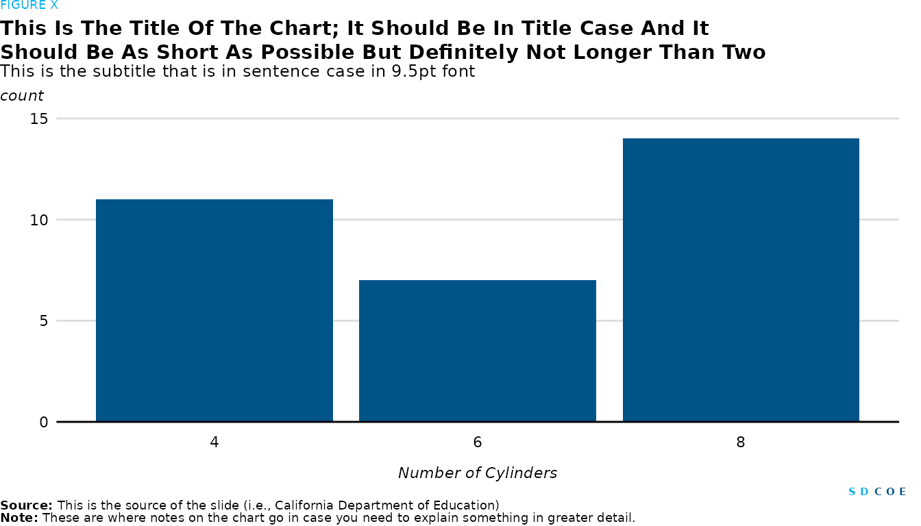
plot <- ggplot(data = mtcars, mapping = aes(factor(cyl))) +
  geom_bar() +
  scale_y_continuous(expand = expansion(mult = c(0, 0.1))) +
  labs(x = "Number of Cylinders",
       y = "") +
  remove_ticks()

sdcoe_plot(sdcoe_figure("FIGURE X"),
                        sdcoe_title("This Is The Title Of The Chart; It Should
                                    Be In Title Case And It Should Be As Short As
                                    Possible But Definitely Not Longer Than Two"),
                        sdcoe_subtitle("This is the subtitle that is in sentence case in 9.5pt font"),
                        sdcoe_y_title("count"),
                        plot,
                        sdcoe_logo_text(),
                        sdcoe_source("This is the source of the slide
                                     (i.e., California Department of Education)"),
                        sdcoe_note("These are where notes on the chart go in
                                   case you need to explain something in greater
                                   detail."),
                        ncol = 1, heights = c(1, 5, 1, 1, 30, 1, 1, 1)
)
# ggsave(filename = "test.png")
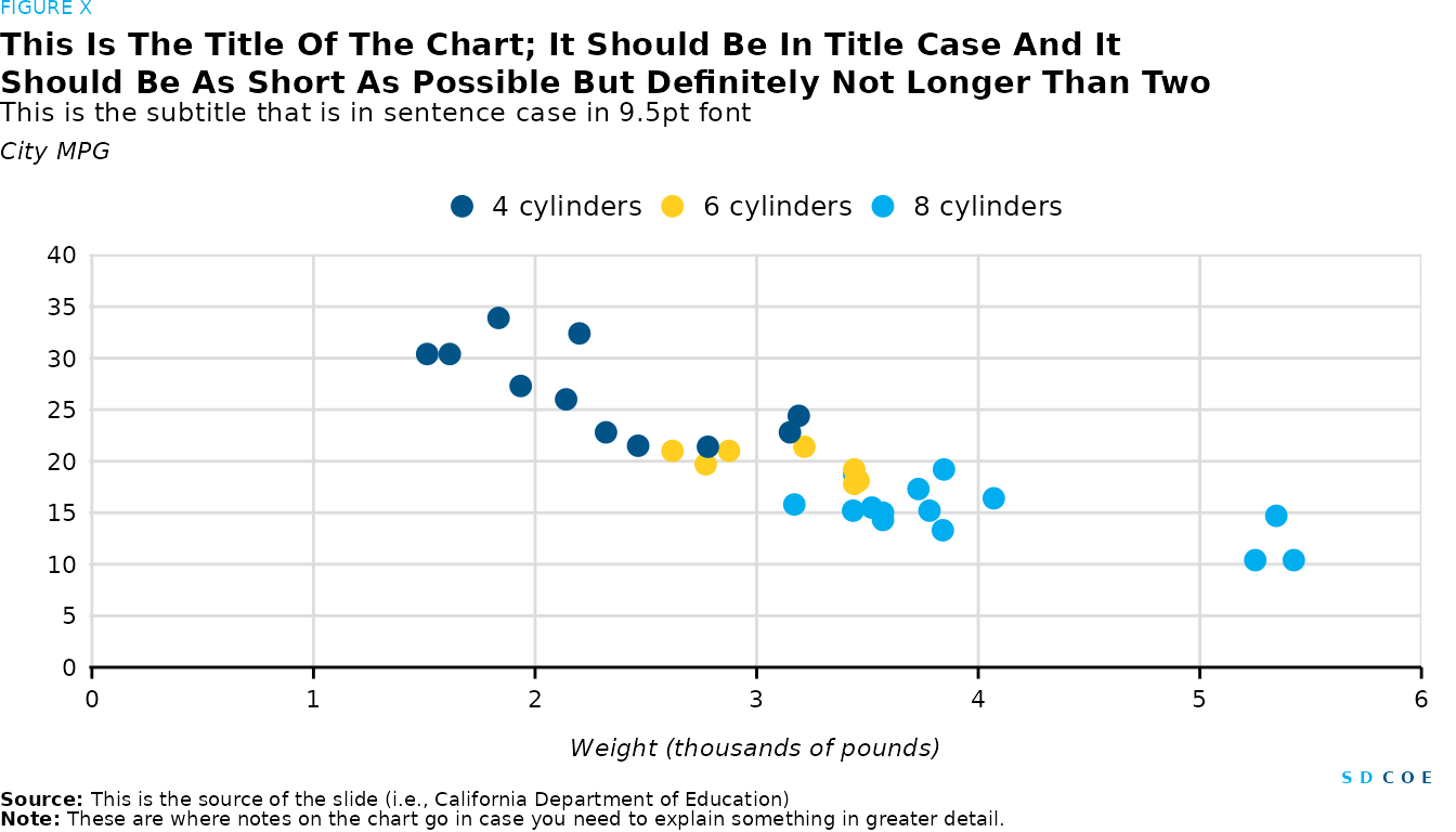
set_sdcoe_defaults(style = "print")

plot2 <- mtcars %>%
  mutate(cyl = paste(cyl, "cylinders")) %>%
  ggplot(aes(x = wt, y = mpg, color = cyl)) +
  geom_point() +
  scale_x_continuous(expand = expansion(mult = c(0.002, 0)),
                     limits = c(0, 6),
                     breaks = 0:6) +
  scale_y_continuous(expand = expansion(mult = c(0, 0.002)),
                     limits = c(0, 40),
                     breaks = 0:8 * 5) +
  labs(x = "Weight (thousands of pounds)",
       y = "") +
  scatter_grid()

sdcoe_plot(sdcoe_figure("FIGURE X"),
                        sdcoe_title("This Is The Title Of The Chart; It Should
                                    Be In Title Case And It Should Be As Short As
                                    Possible But Definitely Not Longer Than Two"),
                        sdcoe_subtitle("This is the subtitle that is in sentence case in 9.5pt font"),
                        sdcoe_y_title("City MPG"),
                        plot2,
                        sdcoe_logo_text(),
                        sdcoe_source("This is the source of the slide
                                     (i.e., California Department of Education)"),
                        sdcoe_note("These are where notes on the chart go in
                                   case you need to explain something in greater
                                   detail."),
                        ncol = 1, heights = c(1, 5, 1, 1, 30, 1, 1, 1)
)
# ggsave(filename = "test2.png")
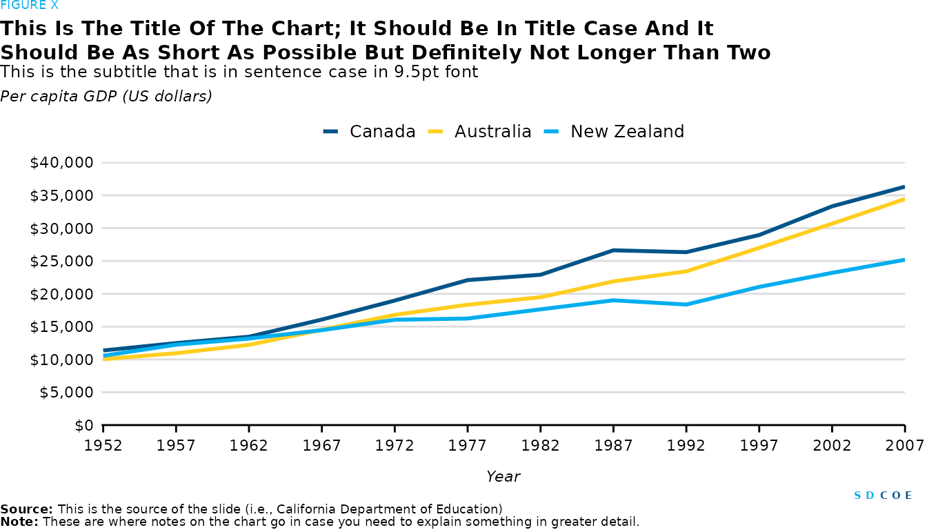
library(gapminder)

plot3 <- gapminder %>%
  filter(country %in% c("Australia", "Canada", "New Zealand")) %>%
  mutate(country = factor(country, levels = c("Canada", "Australia", "New Zealand"))) %>%
  ggplot(aes(year, gdpPercap, color = country)) +
  geom_line() +
  scale_x_continuous(expand = expand_scale(mult = c(0.002, 0)),
                     breaks = c(1952 + 0:12 * 5),
                     limits = c(1952, 2007)) +
  scale_y_continuous(expand = expand_scale(mult = c(0, 0.002)),
                     breaks = 0:8 * 5000,
                     labels = scales::dollar,
                     limits = c(0, 40000)) +
  labs(x = "Year",
       y = "")

sdcoe_plot(sdcoe_figure("FIGURE X"),
                        sdcoe_title("This Is The Title Of The Chart; It Should
                                    Be In Title Case And It Should Be As Short As
                                    Possible But Definitely Not Longer Than Two"),
                        sdcoe_subtitle("This is the subtitle that is in sentence case in 9.5pt font"),
                        sdcoe_y_title("Per capita GDP (US dollars)"),
                        plot3,
                        sdcoe_logo_text(),
                        sdcoe_source("This is the source of the slide
                                     (i.e., California Department of Education)"),
                        sdcoe_note("These are where notes on the chart go in
                                   case you need to explain something in greater
                                   detail."),
                        ncol = 1, heights = c(1, 5, 1, 1, 30, 1, 1, 1)
)
# ggsave(filename = "test3.png")
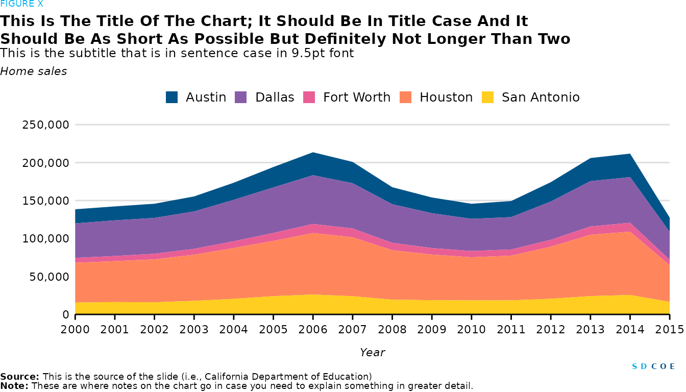
plot4 <- txhousing %>%
  filter(city %in% c("Austin","Houston","Dallas","San Antonio","Fort Worth")) %>%
  group_by(city, year) %>%
  summarize(sales = sum(sales)) %>%
  ggplot(aes(x = year, y = sales, fill = city)) +
  geom_area(position = "stack") +
  scale_x_continuous(expand = expansion(mult = c(0, 0)),
                     limits = c(2000, 2015),
                     breaks = 2000 + 0:15) +
  scale_y_continuous(expand = expansion(mult = c(0, 0.2)),
                     labels = scales::comma) +
  scale_fill_ordinal() +
  labs(x = "Year",
       y = "")

sdcoe_plot(sdcoe_figure("FIGURE X"),
                        sdcoe_title("This Is The Title Of The Chart; It Should
                                    Be In Title Case And It Should Be As Short As
                                    Possible But Definitely Not Longer Than Two"),
                        sdcoe_subtitle("This is the subtitle that is in sentence case in 9.5pt font"),
                        sdcoe_y_title("Home sales"),
                        plot4,
                        sdcoe_logo_text(),
                        sdcoe_source("This is the source of the slide
                                     (i.e., California Department of Education)"),
                        sdcoe_note("These are where notes on the chart go in
                                   case you need to explain something in greater
                                   detail."),
                        ncol = 1, heights = c(1, 5, 1, 1, 30, 1, 1, 1)
)
# ggsave(filename = "test4.png")